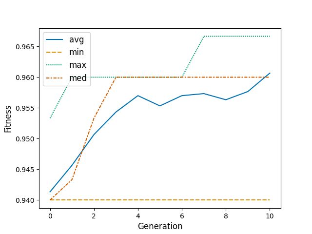
Evolution (logbook) graph

mloptimizer provides a function to plot the evolution of the fitness function.

from sklearn.tree import DecisionTreeClassifier
from mloptimizer.application.reporting.plots import plotly_logbook
from mloptimizer.domain.evaluation import kfold_stratified_score
import plotly
import os
from sklearn.datasets import load_iris
from mloptimizer.interfaces import HyperparameterSpaceBuilder, GeneticSearch
from sklearn.model_selection import StratifiedKFold

Load the iris dataset to obtain a vector of features X and a vector of labels y. Another dataset or a custom one can be used

X, y = load_iris(return_X_y=True)

Define the HyperparameterSpace, you can use the default hyperparameters for the machine learning model that you want to optimize. In this case we use the default hyperparameters for a DecisionTreeClassifier. Another dataset or a custom one can be used

hyperparam_space = HyperparameterSpaceBuilder.get_default_space(estimator_class=DecisionTreeClassifier)

The GeneticSearch class is the main wrapper for the optimization of a machine learning model. Configure genetic algorithm parameters: - generations: Number of evolutionary iterations - population_size: Number of individuals per generation - n_elites: Number of best individuals preserved each generation - seed: Random seed for reproducibility Note: Values reduced for faster documentation builds. For production, use larger values.

genetic_params = {
    'generations': 10,
    'population_size': 20,
    'n_elites': 2,
    'seed': 42
}

cv = StratifiedKFold(n_splits=5, shuffle=True, random_state=42)
opt = GeneticSearch(
    estimator_class=DecisionTreeClassifier,
    hyperparam_space=hyperparam_space,
    cv=cv,
    scoring='accuracy',
    **genetic_params
)

To optimize the classifier we need to call the fit method.

opt.fit(X, y)

GeneticSearch(cv=StratifiedKFold(n_splits=5, random_state=42, shuffle=True),
              estimator_class=<class 'sklearn.tree._classes.DecisionTreeClassifier'>,
              generations=10,
              hyperparam_space=HyperparameterSpace(fixed_hyperparams={'criterion': 'gini'}, evolvable_hyperparams={'min_samples_split': Hyperparam('min_samples_split', 2, 50, 'int'), 'min_samples_leaf': Hyperparam('min_samples_leaf', 1, 20, 'int'), 'max_depth': Hyperparam('max_depth', 2, 20, 'int'), 'min_impurity_decrease': Hyperparam('min_impurity_decrease', 0, 150, 'float', 1000), 'ccp_alpha': Hyperparam('ccp_alpha', 0, 300, 'float', 100000)}),
              n_elites=2, scoring='accuracy', seed=42)

In a Jupyter environment, please rerun this cell to show the HTML representation or trust the notebook.
On GitHub, the HTML representation is unable to render, please try loading this page with nbviewer.org.

We can plot the evolution of the fitness function.

population_df = opt.populations_
g_logbook = plotly_logbook(opt.logbook_, population_df)
g_logbook.update_layout(autosize=True, width=None, height=450)
plotly.io.show(g_logbook, config={'responsive': True})

Alternatively, we can use the simpler plot_logbook function.

from mloptimizer.application.reporting.plots import plot_logbook
import matplotlib.pyplot as plt

g_logbook = plot_logbook(opt.logbook_)
plt.show()

/home/docs/checkouts/readthedocs.org/user_builds/mloptimizer/envs/master/lib/python3.11/site-packages/seaborn/_oldcore.py:1119: FutureWarning: use_inf_as_na option is deprecated and will be removed in a future version. Convert inf values to NaN before operating instead.
  with pd.option_context('mode.use_inf_as_na', True):
/home/docs/checkouts/readthedocs.org/user_builds/mloptimizer/envs/master/lib/python3.11/site-packages/seaborn/_oldcore.py:1119: FutureWarning: use_inf_as_na option is deprecated and will be removed in a future version. Convert inf values to NaN before operating instead.
  with pd.option_context('mode.use_inf_as_na', True):

At the end of the evolution the graph is saved as an html at the path:

print(opt._optimizer_service.optimizer.tracker.graphics_path)
print(os.listdir(opt._optimizer_service.optimizer.tracker.graphics_path))

None
['plot_evolution.py', 'plot_mlp_neural_network.py', 'plot_hist_gradient_boosting.py', 'regression_example.py', 'plot_lightgbm_classifier.py', 'plot_xgboost_example.py', 'plot_catboost_example.py', 'plot_search_space.py', 'plot_xgboost_hyperparam_opt_comparison.py', 'plot_logistic_regression.py', 'plot_lightgbm_regressor.py', 'plot_quickstart.py', 'plot_linear_models.py', 'plot_adaboost.py', 'README.rst']

The data to generate the graph is available at the path:

print(opt._optimizer_service.optimizer.tracker.results_path)
print(os.listdir(opt._optimizer_service.optimizer.tracker.results_path))

del opt

None
['plot_evolution.py', 'plot_mlp_neural_network.py', 'plot_hist_gradient_boosting.py', 'regression_example.py', 'plot_lightgbm_classifier.py', 'plot_xgboost_example.py', 'plot_catboost_example.py', 'plot_search_space.py', 'plot_xgboost_hyperparam_opt_comparison.py', 'plot_logistic_regression.py', 'plot_lightgbm_regressor.py', 'plot_quickstart.py', 'plot_linear_models.py', 'plot_adaboost.py', 'README.rst']